Mehmet Emre Akbulut, Gamze Güliter, Eren Senoglu, Yavuz Samet Topcuoglu

1 Data Description and Preprocessing

Given data is 5200 images having the shape of (96, 96, 3) with RGB channels. Firstly, we started to analyze data in many ways using some visualization techniques in order to gain insight into that data and interpret it. In this period of time, we noticed 2 main things: class imbalance between ‘healthy’ and ‘unhealthy’ and wrong labeled, irrelevant data including ‘shrek’ and ‘trololo’ images. So, we decided to use class weights and remove irrelevant images from every model in the future. Also, as a side note, we noticed that in some images, just a little region with defects leads plants to be unhealthy. Hence, data augmentation is very important for this binary classification problem because for example, if we cut or remove this defected region from the image, it can create unhealthy labeled images without a defected region (so zoom and crop are dangerous to use). So we think this task is flip invariant, not zoom or crop invariant. We briefly made Exploratory Data Analysis to see and interpret data in many ways. With the help of matplotlib and opencv libraries, we can manipulate data, change colors, create charts, pixel histograms etc. You can find thenotebook containing these types of analyses and illustrations. Then, to prepare the data for the learning process, several preprocessing steps were applied:

Normalization:Pixel values were scaled to a range of 0 to 1 for our custom neural network models. For transfer learning, we use that model’s preprocessinput function. Also, with the help of analysis and some sources, we also made pixel histogram equalization.
Data Augmentation: To enhance the model’s generalization capability and robustness, we augmented the training dataset using techniques like rotation and horizontal-vertical flipping to improve model gen- eralizability. These are the safe augmentation techniques we implemented. Apart from these, we tested models if they work well with these techniques: - Gaussian Noise, RandomContrast, RandomBrightness (works well in most cases) - RandomZoom, RandomCrop (not works well - dangerous to use)

We lean towards selecting the model with augmentation and regularization when faced with comparable
success in validation and test accuracy since augmentation and regularization lead to a more generalized
local optimum and a robust solution, in theory. We divided data into 3 sets after using K-fold Cross
Validation, seeing that most of them are similar so we preserve distribution using stratify: training set:
64%, validation set: 16%, test set: 20%.

2 Experiments and Analysis

We conducted a series of experiments and explored various deep learning techniques. Our approach consists of custom-built and pre-trained neural network architectures. This mix allowed us to thoroughly explore the problem space and identify the most effective solutions.

2.1 Custom-built CNNs (from scratch)

As the first approach, we developed a custom CNN based on the architecture we saw in the exercise session to find a balance between model complexity and overfitting. We experimented with different configurations, tweaking layer depths, filter sizes, and dropout rates. The resulting model contains 4 convolutional layers, each with a 0.25 dropout rate, ’ReLU’ activation, and ADAM optimizer. The batch size is 16, and it was trained in 200 epochs with 80% validation and 75% test accuracy. However, this model was too simple for the task, and we decided to move forward with more complex architectures. This custom model helped us to understand which data augmentation techniques can lead to better perfor- mance. Some affected the model with a decrease in accuracy, while others helped increase accuracy. Apart from

this, we applied sampling (up and down) techniques. Even with data augmentation to prevent overfitting, we could not reach better accuracy than the model with class weights (75% on validation generally). So as the final step, we decided to use class weights. Moreover, we found that it would be beneficial to use some preprocessing steps to increase accuracy and create a generalized model. For example, applying gaussian noise and blur with a (5,5) kernel size. Only gaussian noise has increased the validation accuracy to 84%. Also, in the models we manipulate the data, generally, we need more epochs to train because it takes time to fit models to more and various data.

2.2 Transfer Learning

After custom building CNN from scratch, we understand that finding a model with no base ground is very hard to accomplish. Our homemade CNNs have a limited capacity and we need a CNN with more complexity. So we tried alternative architectures starting with traditional ones such as VGG16, MobileNet, and InceptionV3 with the guide ofkeras-applications. As you can see, all of them have different parameter counts. So, working with these models helps us to understand the importance of parameter count, and its effect on training in terms of epochs, training time, and accuracy. Also, we noticed that using more parameters and bigger models does not always lead to better results. We generally use their preprocessing process provided but we also tried reshaping, just giving images with normalization, rescaling etc. Given images with preprocessinput gives the best results in terms of val. accuracy. However, with VGG-16, MobileNet, and InceptionV3 we can not reach more than 80% accuracy (around 78%, 76% and 74% respectively). Also, we saw a tendency to overfit in these models for our dataset, so we discarded them. Moreover, we researched related articles related to transfer learning in binary classification. Inthis article, the models are evaluated by their optimality to a given arbitrary dataset on average. With the help of this article, Xception (extended version of Inception) is our next model giving 89-90% val accuracy and 83% on the submission, which is clearly our best model so far. However, still models do not satisfy us in many ways such as their training time, and overfitting. We also changed the learning rate many times to deal with these problems by using a learning rate scheduler which changes the learning rate after a certain epoch. It helps a bit when it is applied in the correct epoch. Our research comes to an end after readingan article related to EfficientNet. EfficientNetV2M(S) was giving the best results independent of the hyperparameters in our problem and has a tendency to give better accuracy in earlier epochs. Using the same techniques mentioned above we got better results around 87-88% val. , %85-86 test accuracy and started to think about how to improve this specific architecture. We have used Flatten Layer, Dense layers and Dropout which are compatible with our model’s output. Dropouts help us to prevent overfitting. We also observed that having 5 classification layers captures the task’s complexity better than having 1 layer. We tried various values for dropout for each layer but 0.1 or 0.2 gives the best performances, especially 0.2. We have utilized different dense layers starting with various neuron amounts from 1028 to 16. Eventually, we decided to use 5 layers with 512, 256, 128, 64, 16 numbers of neurons (slightly different model to model). At that time, we also changed the output shape and loss functions. We generally prefer the sigmoid function. In the end 88% val. is accomplished. Also, we use L1 and L2 kernel regularizers to prevent overfitting and create generalization. When we have lots of parameters and a small amount of data, penalizing complexity can lead to better results. Eventually, we got 90% accuracy on validation and 87% on submission after fine-tuning by unfreezing after the 85th layer (not final submission, for final just 80-81%). So, apart from EfficientNetV2M(S), we use ConvNeXtLarge as the final submission and it gives us the best result in all phases after fine-tuning the layers (92% on validation and 85.70% on final submission). We used the techniques above because they still improve performance for this model. With the power of ConvNeXtLarge, we tried some ensemble techniques by using 2 models. One of them is an expert to know healthy ones and the other one is unhealthy ones with a 0.7 threshold. However we couldn’t get a result that satisfied us, so we didn’t submit an ensemble model. Maybe using different architectures can help the ensemble, however, we trust ConvNeXtLarge more than other models by far. Model Fine-Tuning:For each architecture, we fine-tuned hyperparameters and layers to better adapt to our specific dataset. The fine-tuning process of the final model is discussed below. These are the general techniques we adopt (used them from the beginning) but we explain them using our specific architecture ConvNeXtLarge.

3 Final Model and Training

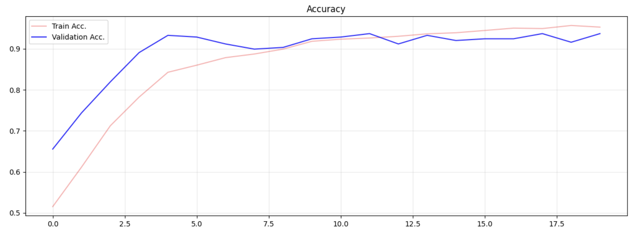
In the end, we utilized the ConvNeXtLarge architecture, chosen for its balance of accuracy and computational efficiency, which is particularly useful for computer vision tasks. Throughout the process of finalizing the ar- chitecture, we followed some best practices to fine-tune hyperparameters for models and validate their success correctly. We used different callbacks:

EarlyStopping: To avoid overfitting. Patience varies, but generally, we used 10% of epochs, typically setting patience to 10.
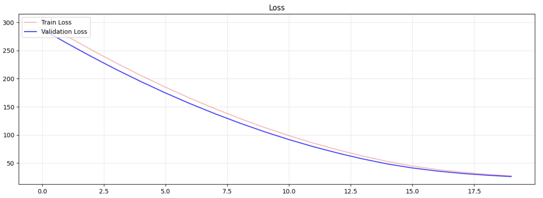
LearningScheduler:To enhance training in the later epochs. Our base learning rate was set to 1× 10 −^5. Additionally, we usedGridSearchto fine-tune hyperparameters and make architecture choices like the op- timizer, dropout rates, etc. This step was not performed in each notebook but rather in the first trial of each different model to capture the best hyperparameters for each base model. We adopted a smaller learning rate and batch size for more stabilized training. The employed learning rate was 1× 10 −^5 , with a batch size of 16, using dropout and L1-L2 regularization to prevent overfitting. Furthermore, we conducted Ablation Studies, systematically altering components such as augmentation techniques and model layers to assess their influence on performance. After observing a substantial gap between the test set and submission scores, we employed these methods. Not only did these methods lead to an increase in accuracy in the test set, but they also reduced the gap in submission scores. In line with theoretical expectations, we observed an increase in generalization in practice as well.

4 Final Notes

Generally, we got very good results with our test sets contrary to submission. We made most of the effort to generalize the model with the help of methods I mentioned above such as architectures, augmentation, and nor- malization techniques (making invariant flip, rotation brightness etc). So there should be distribution differences because still there are features we can not capture. We developed our models to be more generalized and open to different scenarios. ConvNeXtLarge’s accuracy did not decrease compared to others, which makes it the best model we developed.